The diversity of fish is larger than for any other vertebrate group. Not only are there more species of fish (over 31,000) than of all other vertebrates taken together, but also the range of body shapes and sizes of fish is larger than for mammals, birds or reptiles. Consequently, the range of habitats occupied by fishes is larger than those occupied by other vertebrates as well.
The triangle formed by Indonesia, the Philippines and New Guinea, previously referred to as the 'East Indies', form the center of marine fish biodiversity in the Indo-Pacific (Carpenter et al. 2008), with about 2,800 fish species naturally occurring there. These numbers drop with distance from this center to, e.g., about 500 species in Hawaii and 120 species in the Easter Islands. The number of endemic species, i.e., fishes that do not occur outside a given area, increases with distance from the center, which is compatible with the hypothesis that species evolved in the outer region and accumulated in the center. Another hypothesis holds that species evolved in the rich and stable habitats of the East Indies and were carried to the periphery by currents. Randall (1998) gives five explanations for the high fish biodiversity in the Indo-Pacific:
• Sea surface temperatures in the East Indies were more stable during the glacial periods and thus extinction rates were lower than at the periphery;
• Shelf area in the East Indies is much larger than that of the periphery, again making extinctions less likely;
• Dispersal of shore fishes to remote islands occurs during the planktonic larval phase (which lasts from several days to several weeks). However, the larval phase of many species is not long enough for long stretches of open ocean water, thus restricting their distribution;
• Existing current patterns support dispersal of fish larvae from, as well as convergence of larvae of species that have evolved in the periphery towards the East Indies;
• During the last 700,000 years, there have been at least three ice age events that reduced the water level in the East Indies and separated populations long enough for speciation to occur.
• In FishBase, go to Information by Country/Island, select a number of islands along a North-South gradient in the Atlantic or a West-East gradient in the Pacific. Note the latitude or longitude, the area of the island, and the number of marine fishes. Sort the the islands North to South or West to East. Discuss reasons for the observed trends in species numbers. [Hint: Use Country Info to get coordinates and area, use Marine to get species numbers.]
• Use Randall's five explanations to discuss the pros and cons of the 'dispersal from center' versus the 'immigration from periphery' hypotheses.
The relationship between the number of species in an area (i.e., a river basin area, a lake, a shelf area) and the size of the area is known as species-area relationship and implies that the number of species in a given area increases with the size of the area. The latitudinal variation in diversity implies that the tropics are much richer in species than temperate and higher latitudes. These two general trends were the first 'diversity patterns' observed by ecologists for both aquatic and terrestrial ecosystems (see Rosenzweig 1995, Hawkins 2001), and a large number of hypotheses have been proposed for their explanation (e.g., Conor and McRoy 1979, Rosenzweig 1995, Anderson 1998, Hawkins 2001).
The species-area relationship is generally expressed as a power law (Arrhenius 1921) of the form:
S=c·Az 3.1)
which, after logarithmic transformation of both S and A, takes the linear form:
log10(S)=log10(c) + zlog10(A) ... 3.2)
where S is species richness, A is the area of the ecosystem, and z and c are constants. For instance an analysis of a large number of lakes from Africa, USA and Canada, Europe and Asia, tropical Asia and tropical America as well as of rivers from Europe, Asia, Africa and South America (Table 3.1) indicates that, on a log-log plot, species richness was linearly related to lake and river basin area, respectively with the latter explaining more than 67% of the varability in species richness (Amarasinghe and Welcomme 2002). The exponent of the relationship between fish species richness and lake and river basin areas was larger in tropical than in temperate regions, a fact suggesting that freshwater fish species richness increases faster in the tropics than in temperate regions (Amarasinghe and Welcomme 2002).
Table 3.1. The relationships between number of fish species (log10) and river basin area (log10) in different geographical regions (from Amarasinghe and Welcomme 2002)

• FishBase provides a list of All fishes by country (all), and ecosystem (several) (i.e., Information by Country / Island, Information by Ecosystem). Select 10 marine ecosystems of different sizes (area). Get the list of all species and the number of species per ecosystem. Relate this to the area of the ecosystem. [Hint: for the ecosystem area, see http://www.seaaroundus.org/]. Compare the slope of the species-area relationship with the slopes shown in Table 3.1. Discuss the results in the form of a short essay.
• Select five tropical, subtropical, temperate and arctic/antarctic ecosystems (use Information by Ecosystem). Get the list of all species and the number of species per ecosystem. Compare the mean number of species per ecosystem type. [Hint: in Excel you can generate a file with columns entitled Ecosystem and Ecosystem type. Assign the dummy variables, 1 for tropical, 2 for temperate, and 3 for arctic/antarctic ecosystems. Use analysis of variance (ANOVA) from Tools/Data analysis to compare the means.] Discuss the results in relation to the latitudinal diversity pattern in the form of a short essay.
The shapes of fish are also extremely diverse, and include besides the torpedo shape perceived as 'typical' for fishes and termed 'fusiform' shapes ranging from the serpentine (in the Anguilliformes and other orders) to the avian (in 'flying fishes'), with the coelacanth, Latimeria chalumnae sporting limbs resembling, though not being used as, those of land-based tetrapods. Common basic shape categories of fish include: laterally flattened, ventrally flattened, torpediform or fusiform, arrow-like, eel-like, ribbon-like and spheroid shaped (e.g., Nikolsky 1963). Examples of the common categories of fish shapes are shown in Table 3.2.
Table 3.2. Common basic shape categories of fish.
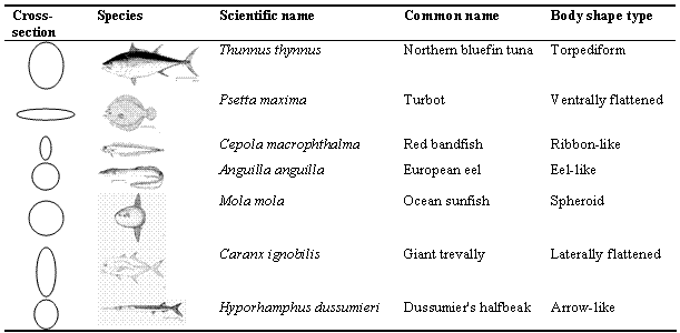
Shape and other morphological features are the key characteristics still used to date for classifying fishes. Hence, understanding the classification of fishes requires a basic overview of their basic shapes. This can be obtained from the outline drawings included in FishBase, for each of the existing 500 fish families.
Body shape plays an important role in the way fish swim, prey and avoid predators and affects the way fish are caught by various fishing gears (e.g., trawls, gill and trammel nets, longlines, traps) and determines the size ranges caught by these fishing gears (i.e., gear size-selectivity; see Stergiou and Karpouzi 2003).
Apart from body shape other external morphological features also exhibit a high variation, e.g., (a) the shape of the caudal fin the main organ, acting with the caudal peduncle, which generates the required thrust for moving in the water can be rounded, truncated, pointed, or forked; (b) the mouth size ranges from small to very large; (c) the mouth shape ranges from an ellipse to a full circle; and (d) the position of the mouth can be inferior, subterminal, terminal, or superior.
• Find from FishBase five species (not from the same genus) exhibiting the basic body shape types shown in Table 3.2. [Hint: use the Identification under Tools]. From the Species Summary page, find the habitat (e.g., pelagic, benthopelagic, demersal) of these species. Can you draw any inference, e.g., on the metabolic activity of the species, from these two sources of information?
• Find five species (not from the same genus) for each main type of caudal fin shape and mouth position. [Hint: use Identification under Tools]. From the Species Summary page, find information on the habitat and diet (from More Information) of these species. Can you draw any inferences, e.g., on the growth of these species, from these sources of information?
The body of fish is usually covered with scales, which provide protection. There are four basic types of scales:
• placoid scales (pointed, analogs of vertebrate teeth, e.g., in Elasmobranchii);
• cosmoid scales (probably evolved from the fusion of placoid scales, e.g., in Family Ceratodontidae);
• ganoid scales (rhomboid shaped, modified cosmoid scales; e.g., in Family Lepisosteidae); and
• elasmoid scales, separated into cycloid (circular with smooth edges) and ctenoid (circular with combed edges) scales, e.g., in Actinopterygii.
Scale size and morphology (especially of elasmoid scales) vary greatly from very small-sizes to highly modified scales (i.e., plates). There are many species that have no scales (e.g., the spotted torpedo, Torpedo marmorata, Family Gobiesocidae) and in some, e.g., flatfishes, scale type varies with sex and location on the body (dorsal vs. ventral).
Scales are of high practical importance to fisheries biology, notably because they (and other skeletal elements such as otoliths and rays) grow as fish grows. This leads to the formation of annual rings on the scales, much like in trees. The age of fish can be estimated from reading the number of annual rings on the scales (see Casselman 1979; Francis 1990). This results in length-at-age pairs which can be used to estimate growth in length (see section 3.8 on Diversity of growth).
• Use Google images to find photos of the different types of scales. Then use the colour photos in FishBase to find several representative species for each scale type, as well as different variations in scale morphology. [Hint: many natural history museums whose collections are searchable online also contain photos of scales and otoliths of fish in their natural history collections.]
Fish are beautiful; they have strange body shapes and vivid colors, the latter a major reason why people keep them in aquaria. Color patterns in fish have been long misunderstood. Some pre-Darwinian authors thought that God had given fish such marvelous colors so that predators would find it easier to see and catch them. We know, since Darwin, that such coloring, if it serves any function at all, must benefit directly the individuals sporting it, and not their predators. This is now obvious in the many color patterns that camouflage their owner, or confuse predators, by, e.g., displaying large eyes in the wrong places. Darwin also proposed a reason why non-camouflaging, striking coloring should exist, and that is sexual selection.
Essentially, the males entice the females to choose them by displaying nicer colors than other males; they compete in terms of their 'beauty', this being related to good genes (remember: Darwin did not know of genes and developing this part of his theory was very difficult for him). Recently, the Zahavi's complemented Darwin's version of sexual selection through a new concept, the handicap principle, which takes into account that the colors and other adornments which males use to entice females are costly to produce (Zahavi and Zahavi 1997). Hence, the color and other adornments represent a 'handicap' and the males capable of displaying these attributes thus should have really good genes for other life-supporting traits. We may call this 'truth in advertisement'.
The idea is that sporting highly symmetrical patterns, as, for example, in the emperor angelfish, Pomacanthus imperator, implies that the fish in question had a harmonious development since development problems, due to genetic problems, parasites or disease (also indicative of 'bad genes') would always lead to asymmetries. In addition, for colors that do not necessarily camouflage the fish, sporting them indicates that the fish in question has been able to evade predators. Some fish, however, imitate the color patterns of other species to fool prey or predators (mimicry), sometimes making them conveniently 'disappear' in the habitat they occupy.
• Read chapter XII, 'Secondary sexual characters of fishes, amphibians and reptiles', in Charles Darwin's Descent of Man, Vol.2. Give a one-page summary of the argument and re-express the main line of Darwin's argument using fish other than the ones in that chapter.
• Give examples from FishBase for species that use color patterns for (a) camouflage, (b) predator confusion, and (c) sexual selection.
• Give one example of mimicry in fishes. Explain the benefits gained. [Hint: common names of such species often contain the words 'mimic' or 'false'.]
• Find from FishBase 10 pelagic species, 10 reef-associated and 10 bathydemersal species. Compare their colouration from the different photos from the Species Summary page and write a paragraph to describe this.
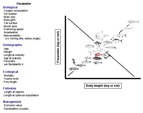
Size is the most important attribute of individual organisms; it determines what can be their food, and the extent to which they can be the prey of other organisms. Size also determines how much food an animal requires, how fast it can swim, and to a large extent, where it can live. In fact, size is related to a plethora of biological, demographic, ecological, fisheries, and management parameters (Figure 3.1), which are often true within and between species. This shows that [...] marine fishes have been shaped by strong constraints, which once overcome, have produced strongly convergent features and hence predictable patterns [...] (Cury and Pauly 2000). In addition, length can generally be easier obtained than any other parameter and thus length records are available in most laboratories studying fish.
FishBase provided the opportunity to explore a large number of the relationships enumerated in Figure 3.1 (see Froese and Binohlan 2000) which illustrates FishBase's capacity to transform information, i.e., each individual points, observations or records, to knowledge, i.e., the form resulting from the relationship of these individual points.
Maximum length (Lmax) is available for the vast majority of species (i.e., for 26,262 species in FishBase as of September 23, 2008). The Lmax of fish ranges from less than 1 cm (e.g., 0.8 cm SL for the plainchin dreamarm, Leptacanthichthys gracilispinis and 1 cm TL for Photocorynus spiniceps) to 1,100 cm TL for the king of herrings, Regalecus glesne, and to 2,000 cm in the whale shark, Rhincodon typus (Figure 3.2). The Lmax appears roughly log-normally distributed, but is actually right-skewed towards large fishes (Figure 3.2; Froese 2006). Fifty percent of fishes have Lmax between 9 and 33 cm, and 90% of fishes between 4 and 96 cm (Froese 2006).
The maximum weight of fish also varies greatly but it is available for much less species (for 1688 species as of September 23, 2008) than Lmax. It varies from about 1 g, such as in the lemon tetra, Hyphessobrycon pulchripinnis, to 4 t for the basking shark, Cetorhinus maximus, and 34 t for the whale shark, Rhincodon typus.
This diversity of size allowed widely different environments to be colonized, ranging from temporary puddles to the central gyres of the open ocean. However, colonizing these environments required other adaptations, involving growth and mortality rates, and their various correlates, discussed in the sections below.
 |
| Figure 3.1. Relationship between length and other parameters in fishes (from Stergiou 2005a). |
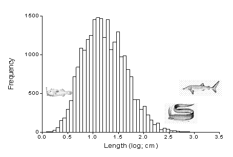 |
| Figure 3.2. Frequency distribution of maximum lengths in 23,685 species of fishes (from Froese 2006). The depicted species are from left to right: plainchin dreamarm, Leptacanthichthys gracilispinis, king of herrings Regalecus glesne, and whale shark, Rhincodon typus. |
• Write down 20 marine and fresh water fish species that you know from your country. Next to the name of each species write its maximum length based on your knowledge or guess. Use FishBase to check your guesses.
The relationship between weight (W) and length (L) in fishes has the form:
W=aLb 3.3)
which after logarithmic transformation of both length and weight takes the linear form:
log10(W)=log10(a) + b·log10(L) ... 3.4)
wherein log10(a) is the intercept and (b) the slope or regression coefficient.
Length-weight (L-W) relationships are very useful for fisheries and ecological research because they are used: (a) to convert growth-in-length equations to growth-in-weight, for stock assessment models; (b) for the estimation of the biomass of a species from length frequency distributions from both onboard surveys and underwater ('eyeballing') observations; (c) as an estimate of the condition of fish; and (d) for between-region comparisons of life histories of a certain species. As a result, L-W relationships are an important component of FishBase (see The LENGTH-WEIGHT Table; Binohlan and Pauly 2000), which, in August 2008, contained 8,049 records for 3,164 species of fishes.
The analysis of a large number of L-W relationships from FishBase (Froese 2006) shows that the values of the slope b generally range between 2 and 4, with 90% of the values ranging from 2.7 to 3.4 (Figure 3.3). Values of b smaller, equal and larger than 3 indicate isometry, negative allometry and positive allometry respectively. When b=3, small individuals have the same shape and condition as large ones. On the other hand, when b>3, large specimens increase in height or width faster than in length, either as the result of a change in body shape with size (an infrequent case), or because the large specimens in the sample are in better condition than the small ones. Conversely, when b<3, either the large specimens have changed body shape, i.e., become more elongated, or the small specimens were in better nutritional condition at the time of sampling. We point out that values of b<2.5 or >3.5 are often derived from samples with narrow size ranges (Carlander 1977; Froese 2006), although there are species with truly and strongly allometric growth (e.g., the red bandfish, Cepola macrophthalma, with an exponent of b~2.0, and the blackfin icefish, Chaenocephalus aceratus with an exponent of b~3.7).
The parameters a and b of the L-W relationship vary with the size range of the sample and thus their use should be strictly limited within this range. They also generally vary with sex, season and area.
The plot of log10a vs. b for all species with available L-W relationships (Figure 3.4) shows that the variation in log10a is largely a function of the body shape of the respective species (Froese 2006). This plot, called 'Froese plot' by Karachle and Stergiou (2008), can be used to identify outliers, i.e., points that deviate from the (straight) regression line.
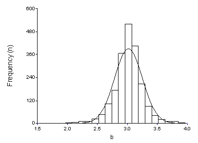 |
| Figure 3.3. Frequency distribution of mean exponent b based on 5,079 records for 2,054 species, with normal line overlaid (from Froese 2006). |
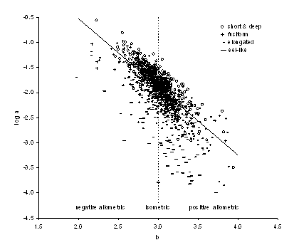 |
| Figure 3.4. Scatter plot of mean log10a (cm; TL) over mean b for 1,232 fish species with body shape information (see legend). Areas of negative allometric, isometric and positive allometric change in body weight relative to body length are indicated. The regression line is based on robust regression analysis for fusiform species (n=451) (from Froese 2006). |
Table 3.3. Mean fork length-at-age of the St. Lawrence River population of muskellunge, Esox masquinongy, adapted from Scott and Crossman (1973, p. 367).
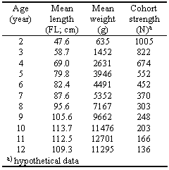
• Based on the data in Table 3.3, estimate the parameter a and b of a length-weight relationship of the form W=a·Lb. The procedure to apply is the linear regression routine in Excel (or another spreadsheet or statistical software) after taking the logarithm of the length and weight observations. Results should be presented with estimates of the precision of the a and b parameters. [Hint: The regression function in Excel is found in the Data Analysis option under the Tools menu.]
• Find one L-W relationship for each species per basic shape type used in exercise 3.3 (Diversity in shapes). Plot on the same graph the theoretical regression lines for the length ranges of all species per shape type, as reported in the LENGTH-WEIGHT Table [Hint: in Excel, generate a series, named Length, starting from 1 up to the maximum length of the largest species you have selected, using step size 1 cm. In the next column, generate a series, named Weight, i.e., for each cell of the weight series, estimate the weight corresponding to each length using the L-W equation available for each species]. Compare the L-W relationships and discuss the results.
• Find from FishBase all L-W relationships of the gila trout, Oncorhynchus gilae, the European hake, Merluccius merluccius and the cod, Gadus morhua. Plot log10a vs. b for all relationships per species. Fit a linear regression to each. [Hint: The regression function in Excel is found in the Data Analysis option under the Tools menu.]. Check for points that deviate from the regression line.
Growth is the increase in size (i.e., length and weight) with time and the change in size per unit of time is called growth rate. The most commonly used equation to describe growth in fishes is the von Bertalanffy growth equation, which has the form:
Lt=L∞ [ 1 e K ( t t 0 ) ] 3.5)
where Lt is the mean length predicted at age (t); L∞ ('L -infinity'), the mean size the fish would reach if they were to grow indefinitely (i.e., for a very long time); K is the rate at which L∞ is approached (with dimension 1/time); and t0 is the (usually negative) age the fish would have at length zero if they always grew as predicted by the equation (which they don't).
The L∞ values estimated for fishes range from 1 cm in some short-lived gobies to around 14 m in long-lived whale sharks, as can be expected given their maximum size (see section 3.6 above). K values range from 8.5 year-1 for small-sized, fast growing species such as the delicate round herring, Spratelloides delicatulus, to 0.02 year-1, for the Adriatic halibut, Hippoglossus hippoglossus.
Parameters of the von Bertalanffy growth function are very important for ichthyology, and fisheries biology and ecology. They are used in life-history studies, in stock assessment and in ecological models. These parameters are usually estimated either from: length-at-age data (directly from readings of daily, monthly or annual rings from skeletal elements, i.e., otoliths and scales,); length-frequency data; or mark-recapture data. For species without available growth parameters in FishBase, e.g., rare species or species which are not exploited by commercial fishing, L∞ can be estimated from the empirical relationship presented in Froese (2000):
log10L∞ = 0·044 + 0·9841 log10Lmax 3.6)
which was based on 551 data sets from FishBase and where the resulting r2 is 0·959 and SE is 0·074).
The VBGF parameter K can be estimated using three different approaches. In cases where there are no VBGF parameters available, maximum age can be used with the empirical relationship:
K≅3/(tmax ) 3.7)
In cases where no growth studies are available, but length at first maturity (Lm) is available with age at first maturity (tm), K can be estimated from the empirical relationship:
K≅loge(1- Lm/L∞)/(tm) 3.8)
where L∞ is estimated using equation 3.6. Finally, in cases where growth parameter estimates are available for different populations or for closely related species, K can be estimated from L∞ through the growth coefficient index (Ø') and the empirical relationship from Pauly et al. (1998):
Ø'=log10K + 2·log10L∞ 3.9)
In spite of the wide diversity of fish sizes mentioned above, clear patterns do emerge. One is that tropical fish tend to be smaller and faster-growing than their cold-water counterparts and that their natural mortality tends to be higher (see section below). This is due to high temperature elevating the metabolic rates of tropical fish relative to their cold-water counterparts (Pauly 1998). Thus, when one estimates the parameter of the von Bertalanffy growth equation in tropical fish, one usually ends up with relatively low values of L∞ and high values of K, at least as compared with their cold water analogs.
• Estimate the von Bertalanffy growth parameters (L∞, K and t0) for the muskellunge Esox masquinongy, based on the age-length data pairs in Table 3.3. [Hints: The von Bertalanffy equation can be linearized through the expression Lt+1 = a+b·Lt wherein Lt and Lt+1 are the length at successive ages. Once a and b have been estimated by linear regression (see section 3.7.1), L∞ and K can be estimated from L∞=a/(1- b) and K =-loge(b); t0 can then be obtained by solving the von Bertalanffy equation for a few Lt and t data pairs and averaging the solutions. Alternatively, a non-linear fitting routine, such as 'Solver', built in Excel can be used to solve simultaneously for L∞, K and t0 (see the Excel manual on how to use Solver).]
• Identify two families, one tropical, one temperate, whose representatives have similar maximum sizes, and compare the distribution of their growth parameters on an auximetric plot.
• Find from FishBase five species, each having more than 10 sets of von Bertalanffy growth parameters. [Hint: use commercial species, check for growth parameters in the Species Summary page, More Information link.] For each species, plot log10K vs. log10L∞. Fit the five regression lines. [Hint: The regression function in Excel is found in the Data Analysis option under the Tools menu.] Compare the five slopes. Discuss the results.
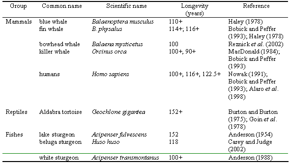
Longevity (or lifespan) is defined as the oldest fish ever recorded for an unexploited species or stock, and can be approximated by the maximum known age. The latter also varies greatly in fishes, from very few months, in, e.g., seven-figure pygmy goby, Eviota sigillata, to 140 years for warty oreo, Allocyttus verrucosus, 149 years for orange roughy, Hoplostethus atlanticus, and 157 years for shortraker rockfish, Sebastes borealis. Fish are exceptional among vertebrates (Table 3.4) in terms of their lifespan. They are characterized by many species with lifespans more than 100 years (Reznick et al. 2002). Reznick et al. (2002) attribute this to the fact that fishes are characterized by 'indeterminate growth' (depicted in the von Bertalanffy growth equation; see section 3.8), which allows for a substantial increase in fecundity with age (see section 4 on Reproduction).
Lifespan is the result of mortality caused by the combined action of intrinsic and extrinsic sources (Partridge and Barton 1996; Reznick et al. 2002). Although lifespan is not synonymous to senescence, long lifespans can only be achieved with the combination of low extrinsic mortality rates and deferred senescence (Reznick et al. 2002).
The loss of individuals due to natural intrinsic and extrinsic causes, such as predation (the main cause of natural mortality), starvation, diseases, genetic anomalies, etc, is known as natural mortality (M). However, humans use fish for food and other purposes (e.g., recreation, aquaria), which cause additional mortality. The mortality caused by all forms of fishing is known as fishing mortality (F). The sum of natural and fishing mortality is called total mortality (Z).
Natural mortality is one of the most difficult parameters to estimate because nowadays most fish stocks, commercial or not, are affected directly or indirectly by fishing. As a result, most of the available estimation methods provide estimates of Z rather than M. Thus M is often estimated from empirical equations, which relate existing M values for several unexploited stocks to other parameters. Two of the most commonly used empirical methods are those of Hoenig (1983), which relates M to maximum age, t max, for unexploited stocks (thus Z=M) and was based on data for 84 stocks of 53 fish species:
logeZ=1.46 1.01·logeTmax 3.10)
Table 3.4. Known supercentenarian vertebrate species (i.e., species with longevity >100 years).
and Pauly's (1980) equation, which relates M to L∞, K and mean temperature (T) in the habitat of the stock and was based on data from 175 stocks:
logeM=-0.0152 0.279·logeL∞ + 0.6543·K + 0.463·loge(T) 3.11)
The natural mortalities experienced by fish, which are also a function of their size and age, range from values which exterminate an entire cohort in less than a year, e.g., in the Lake Tanganyika sprat, Stolothrissa tanganicae (M=5.2 year-1), to values which suggest an average life expectancy of over 20 years, e.g., in the lake sturgeon, Acipenser fulvescens (M=0.06 year-1). These enormous differences in natural mortalities and lifespans allow fish to respond differently to habitat variations. Small, short-lived fish track such variations, for example, when growing up in temporary puddles and laying desiccation-proof eggs before they dry up, thus being able to live through dry periods, or by spawning every year, but producing a successful cohort only once every 5-10 years (as may happen in such long-lived fish as cod, Gadus morhua).
• Reznick et al. (2002) reports 13 fish species with age>100 years. Table 3.4 shows some of them. Find from FishBase as many fish species as possible with ages>100 years and fill Table 3.4. [Hint: Size is related to age. A list of growth parameters available in FishBase can be accessed under the Information by Topic section of the FishBase search page.]
• Estimate the value of natural mortality (M) from the relative abundance in Table 3.3 (4th column). [Hints: M can be estimated as the slope (with sign changed) of the regression of loge(N)= a+b·t, where N is the number of fish in a cohort, and t their age. The regression function in Excel is found in the Data Analysis option under the Tools menu.]
• Compare natural mortality (M) estimates for 10 species of tropical fish, ranging between 50 and 100 cm maximum length, with 10 species of fish with similar sizes from cold waters and test for a temperature effect. [Hint: temperature and M values maybe found in the Life history tool available from the bottom of the Species Summary page.]
• Select 10 commercial stocks (from different species) for which there are available records of maximum age (tmax) and von Bertalanffy parameters. Estimate their natural mortality (M) using Hoenig's (1982) and Pauly's (1980) empirical formulas. Compare and discuss the results.
• Select 30 stocks from different species for which there are records of natural mortality (M), maximum age (tmax) and maximum length (Lmax). Plot log10M vs. log10tmax and log10M vs. log10Lmax. Fit the regression lines. [Hint: The regression function in Excel is found in the Data Analysis option under the Tools menu.] Discuss the results.
Fish inhabit more diverse habitats than any other group of vertebrates, ranging from Himalayan or Andean brooks at 4000 meters to abyssal depth at 10 kilometers, thus spanning an extremely high range of pressures. The range of temperatures that can be tolerated is also very large, from minus 2°C as for the antarctic fish Pagothenia borchgrevinki (which sport anti-freeze substances in their blood; see Eastman and Devries 1985); to up to 40°C for the natron tilapia, Oreochromis alcalicus, which lives at the edge of a hot spring in Lake Nakuru in Kenya. (This does not consider the temperature tolerance of deep-sea vent fishes, which have not yet been studied in detail).
Because fish occur only in habitats which they can tolerate, and tend to be abundant in those habitats to which they are best adapted, occurrence records kept by museums can be used to reconstruct the habitat preferences of fishes whose ecology is otherwise unknown. Such records have been named bioquads because they refer to biodiversity and consist of four key elements: (a) the name of the organism; (b) the place where it was caught; (c) the source or person who sampled or identified it; and (d) the date (Pauly and Froese 2001). FishBase makes wide use of bioquads for documenting the distribution of fish and this can be emulated by ichthyology students who may assemble bioquads from FishBase and other sources, notably the Internet.
• Select a species in FishBase and print a point map as well as the point information. See whether you can find additional points in ichthyological museum collections. Identify problematic records. Infer from the habitat (i.e., occurrence records) or the ecological requirements of that species. [Note: links to point maps are available from the Species Summary page. Point information details are shown by clicking on a point (or dot) in a map.]
• Find from FishBase 20 species inhabiting very deep waters (e.g., bathypelagic, bathydemersal). [Hint: use the Information by Country / Island, Biodiversity, Deep-water link.] Compare their morphology and identify special adaptations in morphology for deep-water life.
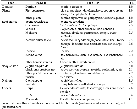
Given the diversity of their sizes and habitats, it is obvious that fish should also have a wide diversity of food and feeding habits. Thus fish range from feeding on microscopic phyto- and zooplankton to engulfing entire adult fishes, such as is done by whale sharks or gulpers, respectively. Attempts to link fish to their ecosystems have led to a huge literature on their food and feeding habits. Unfortunately, some of these are useless because they are reported using the wrong units, i.e., frequency of occurrence of certain items in a number of stomachs sampled. Still, there are enough studies in which the proper units have been used (contribution in weight, energy or volume to total stomach contents) for a clear idea to emerge of what fish generally eat in their typical habitat. Given knowledge of the average trophic level of their diet items (Table 3.5), the trophic level of fish whose stomach content has been studied can thus be computed, which allows evaluation of the position the consumers occupy in the food web (see section 6.1 on Food webs and trophic levels).
Table 3.5. Hierarchy of food items, simplified from the FishBase table used to compute trophic levels (TL) from diet composition data. Therein, the TL of a consumer is 1 + (mean TL of the prey items).
• Find published studies on the diet composition of six different species of fish: two mainly herbivores; two omnivores, and two typical carnivores. Construct a common table including all prey items from all six fish species. In this table the presence of a prey items in the diet of each of the six species is marked with 1 and the absence of a prey species with 0. Subject this table to cluster and multidimensional scaling in order to separate the six species into groups characterised by a similar diet. [Hint: for multivariate analysis use specialised statistical software such as PRIMER]. Discuss results in the form of a short essay.
• Select five species from FishBase and find their main prey items and predators from the Species Summary page (More Information, Prey items and Predators links). For each species construct a simplified food web [Hint: select commercially important species].