7.0 FishBase goes FishBayes

7.1. Traditional vs. Bayesian statistics

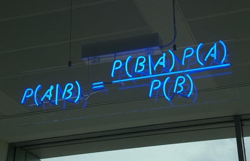
Figure 7.1. The Bayes' theorem (from http://en.wikipedia.org/wiki/File:
Bayes%27_Theorem_MMB_01.jpg).

Traditional statistical methods (also known as frequentist statistics) deal with scientific questions and problems as a de novo procedure without taking into account previous studies and common experience, assuming that the new data to be analyzed cover all the needs of inference. In such an approach, prior knowledge is overlooked and if the new data represent a biased sub-sample, then the results will be misleading. Furthermore, when data are scarce, traditional statistical methods underestimate both physical (i.e., natural variability of a parameter) and technical (i.e., variability derived from methodology such as measurement error) uncertainty associated with the parameters of interest, thus providing unrealistic predictions. At the same time, summarizing all human knowledge and making it easily available to everybody is a long-held human dream. While the Internet and Wikipedia seem to have brought us closer to this dream being realized, the explosion of scientific publications poses new challenges: how do we best summarize several studies dealing with the same topic (e.g., over 50 growth studies for red mullet Mullus barbatus)? How much confidence do we put in a single study? How do we extend knowledge gained from well-studied species (e.g., Atlantic cod Gadus morhua) to understudied ones (e.g., Pacific tomcod Microgadus proximus)?

All the above-mentioned problems and questions can be solved by the use of an 18th century mathematical law: Bayes theorem (Fig. 7.1) or the law of conditional probability. The application of this theorem to complex problems cannot be done analytically because it often results in equations that are too difficult to solve analytically. This difficulty can be bypassed by the use of Markov Chain Monte Carlo (MCMC) simulations, which estimate complex probability distributions empirically. The first algorithm capable of conducting MCMC was published in 1953; the use of Bayesian statistics increased since then. Indeed, the relative frequency of occurrence of the sum of the 2-word phrases (Bayesian inference + Bayesian statistics + Bayesian theory) in the corpus of digitized books increased linearly from 1955 (see Fig. 7.2), following the 1953 publication of MCMC algorithm, up to a plateau during the mid 1970s-1980 and then increased exponentially from 1980 onwards, with the wide use of PCs.

Figure 7.2. Relative frequency of the 2-word phrases (Bayesian inference + Bayesian statistics + Bayesian theory) in the corpus of digitized books. The graph was produced using the Google Ngram viewer, which is available online (http://books.google.com/ngrams).

Statistics are being used in many scientific fields, including fisheries science (e.g., Punt & Hilborn 1997; Varis & Kuikka 1997, Kuikka et al. 1999, Hesler & Lai 2004, Hesler et al. 2004, Haddon 2011, Levontin et al. 2011, Kuparinen et al. 2012). Bayesian statistics are known for their ability to deal with uncertainty based on existing prior knowledge (Winkler 1967). In Bayesian statistics every parameter has to be given a probability distribution. The choice of distribution depends mainly on the nature of the variable modeled and the mathematical convenience of its properties. The normal, log-normal, gamma, poison and beta distributions (Table 7.1) are the most common distributions used in Bayesian analysis, depending on the nature of the problem studied. Bayesian data analysis can be roughly summarized in three steps: First, prior knowledge is quantified in the form of a prior probability distribution for every parameter. Prior knowledge for various parameters can be based either through quantifying the knowledge of experts (expert elicitation) as well as from published studies or other sources (e.g., textbooks). Second, the prior gets updated by how likely the raw data are, called likelihood. Likelihood function is the Bayesian term for the results from analyzing the new data with a certain model. This new knowledge is again expressed as a probability distribution. Third, updating priors with likelihood yields a posterior probability distribution, which is our final probabilistic estimate for the parameters of interest. Posterior probability distribution is the combination of the prior and likelihood probabilities using Bayes’ formula. When we do not have plenty of data the posterior distribution is overwhelmed by the prior distribution. In contrast, when we have a lot of new information, the new data take the leading role in the formation of the posterior distribution.

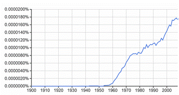
Table 7.1. The most common distributions used in Bayesian analysis (from http://www.mathworks.com, graphs from http://mathworld.wolfram.com).

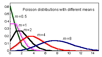	The Poisson distribution is used for modeling rates of occurrence. It has one parameter: m= the rate (mean). Poisson distributions are asymmetric at low mean values, and almost symmetric at higher mean values. When the mean increases toward infinity, the Poisson distribution coincides with a normal distribution. Common usage: For modeling of count data (e.g., number of fish caught in a trawl survey)
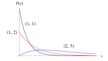	The Gamma distribution is a general distribution covering many special cases, including the Chi-squared distribution and Exponential distribution. It has two parameters: α= rate parameter, β= scale parameter. Common usage: Prior for variance parameters, i.e., from analysis of variance, e.g., of population means.
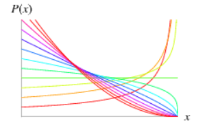	The Beta distribution is a continuous distribution bounded between 0 and 1. It has two parameters: a = first shape parameter, b = second shape parameter When a = b = 1, it is identical to the Uniform distribution on (0,1). Common usage: For modeling rates (e.g., the proportion of individuals that have length smaller than Lm).
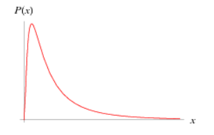	The Log-normal distribution is a continuous distribution in which the logarithm of a variable has a normal distribution. Common usage: Priors of parameters like maximum length, Lm, etc
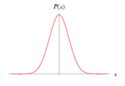	The Normal distribution (also known as Gaussian distribution) is a continuous, symmetric distribution. It is defined by two parameters: the mean (μ) and the variance (σ2). Common usage: Priors of parameters like the exponent of the length-weight relationship.

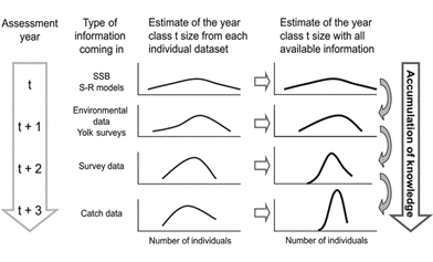
This combination of prior and new information is called scientific learning and is not very different from the way our own brain works. For example, suppose that we know that Atlantic cod Gadus morhua reaches a maximum total length of 150 cm. Suppose now that in a recently published study there is a record of a measured Atlantic cod of 200 cm. Yet, this is just one study. Are we going to abandon our beliefs regarding Atlantic cod’s maximum length? Of course not, we still need more proof. Let’s say now that 20 more studies claim that Atlantic cod does reach 200 cm. Now it is time to leave behind our past beliefs and move towards the new information. The increasing popularity of Bayesian methods is partially attributed to the fact that they make good use of existing knowledge in the form of prior probability distributions, which makes up for lack of data and permits predictions (Winkler 1967; Carlin and Louis 2000). Thus, these methods are especially useful in data-poor situations.

[1] Bayes' theorem is named after Thomas Bayes (/ˈbeɪz/; 1701–1761), who first suggested using a theorem to update beliefs. His work was significantly edited and updated by Richard Price before it was posthumously read at the Royal Society. The ideas gained limited exposure until they were independently rediscovered and further developed by Pierre-Simon Laplace, who first published the modern formulation in his 1812 Théorie analytique des probabilités (http://en.wikipedia.org/wiki/Bayes'_theorem).

[1] Michel et al. (2010) constructed a corpus of digitized books (making up 6% of all books ever printed: Lin et al. 2012) and, using the percentage of times a word/phrase appears in the corpus of books, investigated cultural and other trends. The corpus of books is available in eight languages: English, Spanish, German, French, Russian, Italian, Hebrew and Chinese. Michel’s et al. (2010) computational tool (see also Lin et al. 2012), the Google Ngram viewer, is available online (http://books.google.com/ngrams). This tool estimates the usage

7.1.1. A few more words on priors.

Figure 7.3. A schematic draft of how the Bayesian approach works with new data sets coming in for a year class estimate over time. See text for explanation. The same idea can be applied to, for example, meta-analysis from the literature (different t being different publications).

The use of prior probability distributions is the cornerstone of Bayesian statistics, although it should be mentioned that the subjectivity inherent in this has raised issue (Bayarri and Berger 2004; see also Wasserman 2000). Priors used in Bayesian analysis can be divided in two categories: uninformative (called objective or sometimes “vague”) and informative (or subjective) priors. Uninformative priors carry no information for the modeled parameter. The most commonly used uninformative priors are a uniform distribution with a wide range of values (see Table 7.1) or a normal distribution centered around zero and very high standard deviation. When uninformative priors are used in a model, estimates are identical to the ones taken from traditional methods such as maximum likelihood estimation. This is the huge advantage of Bayesian statistics: they include all other statistical methodologies as a special case. If new data become available, the posterior knowledge from a previous Bayesian analysis is treated as prior knowledge and the process starts all over (Fig. 7.3). In this way, the latest analysis incorporates all previous knowledge. In other words, it is the best available knowledge on a given topic.

7.1.2. Tools used in Bayesian data analysis

Bayesian data analysis is most commonly run through the R statistical environment (http://www.r-project.org/). R is an open source statistical software developed and updated by the users themselves. R includes packages for almost all statistical analyses available today. There are plenty of textbooks for learning R (e.g., the introduction to R, written by the authors of R: http://cran.r-project.org/manuals.html; see also http://www.r-project.org/doc/bib/R-books.html, for other books related to R). To perform Bayesian analyses, one also needs a software performing MCMC. The most widely used ones are JAGS (http://mcmc-jags.sourceforge.net/), WINBUGS (http://www2.mrc-bsu.cam.ac.uk/bugs/winbugs/contents.shtml) and BUGS (http://www.mrc-bsu.cam.ac.uk/software/bugs/), all available for free and ready for use within the R environment by loading the corresponding packages. There are also many manuals and textbooks for learning how to use the above-mentioned three packages (e.g., http://sourceforge.net/projects/mcmc-jags/files/Manuals/).

7.2. Examples of Bayesian applications to fisheries research

7.2.1. Length at maturity - Using prior knowledge

Let’s assume that we want to predict the dynamics of the European hake Merluccius merluccius stock in Greek waters. A very important biological parameter, strongly affecting the resilience to overfishing of a population, is the length at first maturity (Lm), which is required as an input to almost all fisheries models. Unfortunately, we only have 3 estimates on the Lm of the European hake from our study area, with mean μ = 35 and standard deviation σ = 5 (Fig. 7.4b). But can we be confident that the mean and standard deviation of these 3 values correspond to the range of values Lm can take? Keeping that in mind, we will go Bayesian and use 3 different ways of quantifying existing knowledge under the form of a probability distribution in order to use it as a prior, mix it with our data and get a posterior distribution for Lm. The first ‘cheap’ option is to search FishBase and extract all available records on the Lm of European hake. By analyzing all the available values, we find that they can sufficiently be described by a normal probability distribution with mean μ = 34 cm and standard deviation σ = 4 [N (34, 4)] (Fig. 7.4a, red color). If we have plenty of time and the suspicion that FishBase does not include all published estimates (e.g., does not include recent studies, gray literature such as PhD and MSc theses, technical reports, conferences proceedings, local journals), we can do our own literature survey using online tools (e.g., Web of Science, Google, Google Scholar, Scopus). Let’s say that our literature search produced new published estimates, which together with those in FishBase, can also be described by a normal probability distribution, but with mean μ = 37 cm and standard deviation σ = 2 [Ν (37, 2)] (Fig. 7.4a, green color). If we have more time and extra resources we can also elicit experts (i.e., scientists who work on the reproduction of European hake) by arranging interviews in which we ask them what they think is the most probable Lm value for European hake. Then, we adjust their answers into a normal probability distribution with mean μ = 39 cm and standard deviation σ = 1.5 [Ν (39, 1.5)] (Fig. 7.4b). We can observe that the prior distribution elicited from experts is more precise (Fig. 7.4c, blue color) but requires more time and money for its estimation. By applying Bayes theorem and mixing our data with each of the 3 prior distributions we get 3 corresponding posterior distributions (Fig. 7.4c).

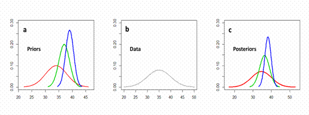
Figure 7.4. Prior probability distributions (a), data (b) and resulting posterior probability distributions (c) for the hypothetical example of length at first maturity (Lm) of European hake Merluccius merluccius. In red and green colors are prior and posterior probability distributions for the FishBase values only method and the method of including new values from a literature survey. In blue color are the distributions derived using expert elicitations.

As you can see posteriors are quite similar to priors. Posteriors, as we say, are overwhelmed by the priors. This happens because of the very small sample size of our data and it makes perfect sense. The model does not trust the estimate from 3 values only and takes more into account prior knowledge. To sum up, we have three different methods of quantifying existing knowledge into three different prior distributions, resulting in three different prior distributions, varying in the level of precision and information they carry, but also in time and money costs spend to obtain them. Note, however, that in a real world situation we could use extra information to increase our knowledge regarding Lm. For example, the Lm of fish of different populations correlate strongly with their maximum length (Froese and Binohlan 2000) and hence we could use that pattern when performing our analysis.

7.2.2. Fitting the von Bertalanffy growth model using prior knowledge

Table 7.2. An example of length (cm) at age (year) for the female Mullus barbatus stock in Tyrrhenian Sea, obtained through otolith readings (from Sieli et al. 2011).

Age	Length
1	109
2	12.1
3	15.2
4	17.2
5	18.4
6	20.2
7	19.8

Let’s now try and fit the von Bertalanffy growth model to some real case data, e.g., mean length-at-age data (Table 7.2) for female red mullet Mullus barbatus stock in the Tyrrhenian Sea (Sieli et al. 2011), using the R statistical environment. First, we will fit the model using a classical least square non-linear regression, which is nowadays the most widely used method in fisheries research. Then we will use a stronger and more modern approach: we will fit a Bayesian model using the existing knowledge on the growth of red mullet, i.e., using all the available data from FishBase. In this way we can search for inferential advantages resulting from the fully Bayesian analysis. The R code needed for fitting the von Bertalanffy equation to the data in Table 7.2 is listed below. This code can be copied and executed in R provided that (a) the R2Jags package is installed; (b) the working directory is set to a folder of your choice in your PC; (c) FishBase growth data for red mullet (Table 7.3) have been copied and saved as a tab delimited file (txt file) under the name ‘FishBaseMullusBarbatus.txt’ in your working directory. To do so, copy both variable names and data in Table 7.3 and paste them in Excel and use the ‘save as’ option to save it as a tab-delimited file.

Table 7.3. All available records of von Bertalanffy growth parameters for red mullet Mullus barbatus in FishBase (L_∞ in cm, K in 1/year, t₀ in years).
L_∞	K	t_o	L_∞	K	t_o	L_∞	K	t_o
17.80	0.19	NA	20.00	0.57	NA	22.40	0.28	-1.98
18.10	0.50	-0.18	20.50	0.50	-0.04	22.50	0.22	NA
18.50	0.63	NA	20.50	0.40	NA	22.50	0.56	NA
19.00	0.59	NA	20.60	0.70	NA	22.70	0.25	-1.13
19.00	0.44	-0.78	21.10	1.09	NA	23.00	0.64	NA
20.00	0.82	NA	21.50	0.27	NA	23.10	0.51	NA
20.00	0.44	NA	22.10	0.23	-1.81	23.50	0.51	-0.86
23.60	0.18	-3.01	24.50	0.60	NA	25.40	0.21	NA
24.00	0.20	NA	24.50	0.14	NA	25.50	0.21	-2.13
24.00	0.26	NA	24.50	0.27	-1.85	26.00	0.41	-0.40
24.00	0.45	NA	24.70	0.15	NA	26.10	0.13	-3.54
24.30	0.57	NA	24.70	0.15	-3.21	26.50	0.16	-2.70
24.30	0.15	-3.31	24.80	0.29	NA	26.60	0.18	-2.49
27.00	0.70	NA	28.30	0.17	NA	29.10	0.41	-0.39
27.50	0.50	NA	28.60	0.15	NA	29.70	0.21	NA
27.60	0.15	-2.64	29.00	0.60	-0.10	31.60	0.11	-2.87

7.2.2.1. R code for fitting the von Bertanffy

###Setting your working directory################# setwd("………..") ##Loading available K and Loo estimates from studies included in Fishbase### FishBaseData<-read.table("FishBaseMullusBarbatus.txt",header=T) FishBaseData ##Entering mean length at age data from Sieli et al. 2011 Age<-c(1,2,3,4,5,6,7) Length<-c(10.93,12.1,15.23,17.24,18.36,20.18,19.77) ###### METHOD 1############## ##Fitting the von Bertalanffy growth model with least square non linear regression##### ##Setting the von Bertalanffy growth model equation## vonBertalanffy<-Length~Loo*(1-exp(-K*(Age-To))) ###Setting initial values for the 3 parameters of the model##### InitLoo<-max(Length) InitK<-mean(FishBaseData$K) InitTo<-0 ##Running the non linear regression model## NLRBertalanffy<-nls(vonBertalanffy,data=list(Age=Age,Length=Length),start=list(Loo=InitLoo,K=InitK,To=InitTo)) ######METHOD 2 ###### ######Fitting the von Bertalanffy growth model with Bayesian inference using previous knowledge### #### Fitting normal distributions to available FishBase data for using them as priors. Log-normal distributions could also be fitted, but let’s stick with the simpler normal distribution for better comprehension. ##### library(MASS) PriorLoo<-fitdistr(FishBaseData$Loo,"normal") PriorK<-fitdistr(FishBaseData$K,"normal") ###Printing the fitted distributions PriorLoo PriorK library(R2jags) runif(1) #######Writing the Model in Jags notation##### Model = "model { for( i in 1 :Nobs){ Length[i] ~ dnorm(mu[i],tau) mu[i]<-Loo*(1-exp(-K*(Age[i]-To))) } ####Setting our informative priors for K and Loo as estimated above##### Loo ~ dnorm(24.9,0.055) K ~ dnorm (0.368,22.3) ####Using an uniformative prior for To and variability at the individual level##### tau ~ dgamma(0.001,0.001) To ~ dnorm (0,0.0001)}" #Saving the model file in the working directory# cat(Model, file="Model.bug") ####Defining data##### DataJ <- list(Age=Age,Length=Length,Nobs=length(Age)) ##Running the model in Jags####### Jags <- jags(model.file="Model.bug", working.directory=NULL, data=DataJ, parameters.to.save=c("K","Loo","To"), n.chains=3,n.thin=10, n.iter=20000, n.burnin=10000) #####Getting results from the jags model###### Jags$BUGSoutput$mean$K #####Getting results from the non linear regression###### summary(NLRBertalanffy) #####Plotting our results##### K_NL<-coef(NLRBertalanffy)[2] K_Jags<-Jags$BUGSoutput$mean$K Loo_NL<-coef(NLRBertalanffy)[1] Loo_Jags<-Jags$BUGSoutput$mean$Loo sd_K_NL<-summary(NLRBertalanffy)$coefficients[2,2] sd_K_Jags<-Jags$BUGSoutput$sd$K sd_Loo_NL<-summary(NLRBertalanffy)$coefficients[1,2] sd_Loo_Jags<-Jags$BUGSoutput$sd$Loo a1<-Loo_NL-3*sd_Loo_NL a2<-Loo_NL+3*sd_Loo_NL b1<-K_NL-3*sd_K_NL b2<-K_NL+3*sd_K_NL xK<-seq(b1,b2,length.out=200) xLoo<-seq(a1,a2,length.out=200) par(mfrow=c(1,2)) ######Plotting posterior distribution of K from Jags###### plot(xK,dnorm(xK,mean=K_Jags,sd=sd_K_Jags)/100,type="l",lwd=1,xlab="K",ylab="") ######Adding distribution of K from non linear regression#### lines(xK,dnorm(xK,K_NL,sd_K_NL)/100,lty=3) ######Plotting posterior distribution of Loo from Jags###### plot(xLoo,dnorm(xLoo,Loo_Jags,sd_Loo_Jags),type="l",lwd=1,xlab="Loo",ylab="") ######Adding distribution of K from non linear regression#### lines(xLoo,dnorm(xLoo,Loo_NL,sd_Loo_NL),lty=3) jpeg("PlotNLvsBayesianGrowth.jpeg") par(mfrow=c(1,2)) ######Plotting posterior distribution of K from Jags###### plot(xK,dnorm(xK,mean=K_Jags,sd=sd_K_Jags)/100,type="l",lwd=1,xlab="K",ylab="") ######Adding distribution of K from non linear regression#### lines(xK,dnorm(xK,K_NL,sd_K_NL)/100,lty=3) ######Plotting posterior distribution of Loo from Jags###### plot(xLoo,dnorm(xLoo,Loo_Jags,sd_Loo_Jags),type="l",lwd=1,xlab="Loo",ylab="") ######Adding distribution of K from non linear regression#### lines(xLoo,dnorm(xLoo,Loo_NL,sd_Loo_NL),lty=3) dev.off()

Running the code listed above in R gives the estimated parameters from the two methods, along with a graph of their distribution (Fig. 7.5). As you can see, both K and L∞ posterior distributions from the fully Bayesian analysis are more informative, since they are characterized by lower standard deviation. Hence, the use of previous knowledge, available in FishBase (Table 7.3), helped us derive more accurate predictions.

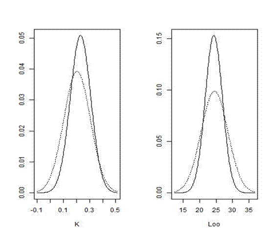
Figure 7.5. Posterior distributions (solid lines) from the Bayesian analysis plotted with non-linear regression estimates (dashed lines) for K and L∞ parameters of red mullet (Mullus barbatus) in the Tyrrhenian Sea.

7.3. FishBase and Bayesian inference

7.3.1. Estimating the maximum sustainable yield (MSY) from catch and resillence: the Catch-MSY Tool

Figure 7.6. Example results of the Catch-MSY Analysis using the FishBase online tool for the target species in the target area (herein the Atlantic cod Gadus morhua in Eastern Baltic Sea).

In FishBase, the Bayesian type of thinking is used in the Catch-MSY online tool, which is available in the ‘Tools’ section in the front page of FishBase. This tool combines catch data with life history traits (e.g., growth, mortality or resilience) and estimates population parameters and fisheries reference points, such as the maximum sustainable yield, MSY (Martell & Froese 2013). The MSY is an important reference point in the exploitation of living aquatic resources. It is the theoretical maximum catch that can be taken from an exploited population (= a stock) indefinitely. Rebuilding and maintaining stocks at sizes that can produce MSY is a binding requirement under the Law of the Sea and in many national legislations. Such a stock size is also called BMSY, i.e., the smallest biomass (B) that can still deliver MSY. Estimation of MSY and BMSY typically requires time series of stock biomass, i.e., annual estimates of the weight of the fish in the sea. Such data are difficult to obtain and are therefore lacking for most of the stocks in the world. The Catch-MSY online tool uses the method proposed by Martell & Froese (2013), which derives a reasonable estimate of MSY from catch data and life history traits, the latter derived from FishBase. Although Martell & Froese’s (2013) approach does not mention Bayes, it is de-facto a Bayesian approach because of the Monte Carlo method and the fact that the priors for maximum intrinsic rate of population increase r and carrying capacity k have uniform distributions. In other words, a formal Bayesian approach would have given identical results.

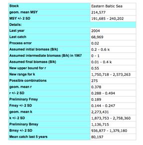
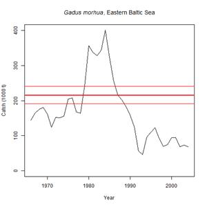
For the application of the Catch-MSY tool, one needs to know the scientific name of the species, a time series of representative catch data for preferably more than 10 years, and a reasonable guess about the stock status at the beginning and the end of the time series. The method will then randomly select several thousand combinations of k and r. It will discard all r-k combinations that let the stock either crash or overshoot the carrying capacity of the system. From the remaining "viable" r-k combinations it will calculate MSY with 95% confidence limits. The whole estimation is completed in the following 5 steps in which the user:

selects the target species and provides a reasonably long time series of catch data;
selects proxies for resilience of the target species in the target area (e.g., in this example Gadus morhua in the Eastern Baltic Sea). This step uses empirical relations between life history traits to obtain preliminary estimates of r: either as r or from estimates of natural mortality (M), or from the von Bertalanffy parameter K, or from the resilience estimate shown in the lower part of the ‘Species Summary’ page by selecting an appropriate resilience category from the choice field that is provided (i.e., Very Low, Low, Medium, High);
verifies the initial ranges for r and k for the selected species (in this example Gadus morhua in the Eastern Baltic Sea). Based on previous entries, the tool provides potential ranges for possible r-k combinations, to be considered by the algorithm, which can be changed by the user;
provides best guess about stock status (in this example for Gadus morhua in the Eastern Baltic Sea); and
sets the process error and number of iterations.

The results are summarized in the form of one Table and six graphs (see an example output in Fig. 7.6). The parameters and reference points are updated whenever knowledge about life history improves or another year of catch data is added.

7.3.2. Bayesian analysis of length-weight relations (LWR)

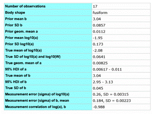
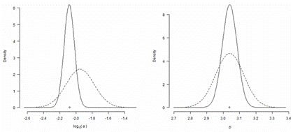
In FishBase, the Bayesian approach has been also used in the analysis of length-weight relations (LWR) for estimating LWR for species for which this information is not available (Froese et al. 2014). FishBase currently holds over 5,000 LWR records for over 1,800 species. The results of the analysis are shown in Table 7.4. Only 410 species had five or more LWR studies, which were used to obtain the best-summarized parameters for the respective species. Seven hundred species had 1-4 LWR specific estimates and five or more species with LWR studies and with the same body shape in their Genus, and then this information was combined in a hierarchical Bayesian approach to obtain a best LWR estimate with confidence limits. If not enough species with LWR estimates were within the same Genus, then relatives in the same Subfamily or Family were included in the analysis. Finally, if there were no LWR estimates for the respective body shape in the Family, then the overall LWR estimates for this body shape were assigned to the species, obviously with wide probability distributions to express the higher uncertainty associated with this case. By this procedure, best LWR estimates could be assigned to 31,872 species. Seventy percent of these estimates were based at least on relatives with the same body shape or on LWRs for the species.

Table 7.4. Best estimates of length-weight relations (LWR) for 31,872 species using Bayesian inference. The ranking indicates the uncertainty associated with the estimate, based on the data that were used, with Rank 1 using only LWR for the target species and Rank 6 using data from species with similar body shapes (from Froese et al. 2014).
Rank	Based on LWR estimates	Number of species
1	for this species	410
2	for this species and Genus-body shape	700
3	for this species and Subfamily-body shape	1,419
4	for relatives in Genus-body shape	1,222
5	for relatives in Subfamily-body shape	18,410
6	for other species with this body shape	9,711

Figure 7.7. Results of Bayesian analysis of length-weight parameters for Atlantic cod Gadua morhua, using the FishBase tool ‘Bayesian analysis’.

Note also that the Bayesian inference approach established a self-learning system in FishBase. Best LWR estimates for all species are updated with every new upload of FishBase. A preliminary analysis of the first update showed that new LWRs added for 16 species resulted in an improvement of Rank in Table 1 for over 400 species. Bayesian analysis of LWR is presently available as a FishBase tool from the ‘Species summary’ page, from where you select ‘Length-weight’ from the heading ‘More Information’. Then from the ‘Length-Weight Parameters’ page you select ‘Bayesian analysis’ (at the bottom of the page). This brings you in the page ‘Bayesian analysis of length-weight parameters for … ’ (in this example for Atlantic cod Gadus morhua: Figs. 7.7 to 7.9). This routine will conduct a Bayesian analysis of the selected length-weight relationships to obtain posterior distributions for the parameters a and b of the length-weight relationship, the measurements of their variance and covariance (Figs. 7.7 and 7.8). The user can select the studies he/she wants to include in the analysis and give them a weight based on their perceived reliability. This can be done by examining the log(a)-b plot for the target species (Fig. 7.9), in which, data points far from the regression line are potential outliers and should thus be given a lower score.

Figure 7.9. Log(a) over b plot with indication of regression line for the target species. Points far from the line are potential outliers and should be given a lower score.

7.3.2.1. Exercises

Ask 20 fishers in your country about the maximum length of the 3 most commercially important fish species in your area. Plot a normal distribution with mean and standard deviation equal to the average and the standard deviation of the data derived from the answers. Do the same thing for all L∞ values available for these three species in FishBase. Is there any difference between the distributions derived from fishers’ and FishBase records? Which prior is more informative? (Tip: as standard deviation increases, the amount of information carried by the distribution is reduced).
Find a long time series of landings (>15 years) for each of the 3 most commercially important species in your area. Apply the MSY tool and write a 3-page essay discussing the implications of your MSY estimates for the management of the species (structure your essay as a scientific paper, i.e., introduction, material and methods, results, discussion, references).
Use the FishBase tool for the Bayesian analysis of length-weight parameters for two well-studied species (>20 length-weight parameters in FishBase) in your country. Do the same thing for a species in your country with very few available length-weight parameters (<3 length-weight parameters in FishBase). Did the number of available data reduce the uncertainty around the length-weight parameters for the two well-studied species? Write a 2-page essay summarizing the results.
Using Google Scholar (http://scholar.google.com/) find an article presenting length at age data for a well-studied species in terms of growth (>20 records of growth parameters in FishBase). Using the code provided in section 7.2.3 fit the von Bertalanffy curve with the two methods described therein. Was there any advantage using the available knowledge in FishBase?